Abstract
This paper introduces a novel digital geopositioning model. It is based on computational geodesy in which direction cosines are used instead of the conventional -angular- ellipsoid normal representation, and eccentricity term expansions are replaced by iterative algorithms. The surface is partitioned by a spheroid equivalent of the Voronoi polygon network. The model affords seamless global coverage, easily attainable millimetric resolution, and data-density sensitive location indexing. Numerical representation of 0, 1 and 2 dimensional objects is in complete accordance with the unbounded, spheroidal nature of the data domain, free from any size, shape or location restriction. Efficient union and intersection evaluations extend the utility of the relational technique into the realm of geometronical systems with non-trivial spatial precision requirements. Digital modelling of orbital dynamics follows closely the numerical methodology used by terrestrial geometry. The Hipparchus software package includes the transformations and utility functions required for efficient generation of transient graphics, and for the communication with systems based on conventional cartographic projections.
A numerical geopositioning model is an essential element of any system wherein a dimension of space enters into the semantics of the application - and therefore into the software technique repertoire - in a fundamental way. It consists of location attribute data definitions and computational algorithms, which allow position sensitive storage and retrieval of data, and provide a basis for evaluation of spatial relationships. (The term "spatial relationship" is used in this paper to describe the formal statement of any practical spatial problem which deals with positions of real or abstract objects on - or close to - the Earth surface. Their nature can vary; examples might include geodetic position computations, course optimization for navigation in ice-infested waters or determination of the most probable location of objects remotely sensed from a platform in the near Space.)
If the location attributes of data elements in a computer system are used exclusively for the generation of a small-scale analog map document, the demands made of a geopositioning model are few and simple. When the area of coverage is limited, and projection geometry, spatial resolution and partitioning of the data can be made directly compatible with same characteristics of all future required products, a single plane coordinate system is often employed. Such a system is usually based on one of the large-area conformal projections (e.g. Lambert, Gauss-Krueger, etc.), and provides adequate means to identify positions, partition the data, and construct a location index. The model may even allow limited spatial analysis.
However, with the increase of the area of coverage and the functional power of information systems, the nature of the problem changes considerably.
Precision requirements usually exceed the level of difference between planar coordinate relationships and the actual object-space geometry. In most cases, the generation of an analog map is reduced to a secondary objective. Location attributes are primarily used to support the evaluation of spatial relationships required by the application. Indeed, as the volatility and volume of data grows, it becomes increasingly common that a location-specific item enters a system, contributes to the evaluation of a large number of spatial relationships, and is ultimately discarded, without ever being presented in the graphical form.
Even in systems used primarily to automate the production of analog documents, there is often a need to accommodate many different projection, resolution and data partitioning schemes on a continental or even global scale.
A point is thus quickly reached where geopositioning model must satisfy very demanding functional requirements, yet any restriction on the data domain becomes unacceptable. From the application point of view, the mapping from an atomic surface fraction into a distinct internal numerical location descriptor must be global, continuous and conjugate.
Faced with these requirements, manual spatial data processing resorts to a combination of two techniques. A set of multiple planar projection systems (e.g. UTM "zones") is used to achieve - seldom successfully - the global coverage. Initially simple calculations are cluttered with various "correction" terms in order to deal with differences between planar coordinates and true object geometry.
A failure to understand the precise nature of spatial data (especially, by ignoring the profound conceptual difference between an analog map and the true data domain) often leads to a blind transplant of conventional cartographic techniques into a computerized system. This seldom results in a satisfactory geopositioning model: cartographic projections are notorious for their computational inefficiency; global coverage usually requires the use of location-specific transformations. Programming becomes progressively more complex as the precision requirements increase. Boundary problems are difficult to solve; this imposes discontinuities or size restrictions for the models of spatial data objects. Finally, classical cartography offers little or no help in modelling of the near-space geometry. The same system can therefore be forced to employ two disparate numerical methodologies: one for the positions on the Earth surface and quite another for orbital data. This presents an increasingly serious problem in many emerging high data-volume applications.
Design (or selection) criteria for a generalized location referencing numerical model and software will change from one computerized information system to another, but will be based - usually - on the size of the area of interest, spatial resolution, anticipated data volume, optimal computational efficiency, logical and geometrical complexity of objects modelled, and on the level of precision with which all these elements can be defined before the system is built. Nevertheless, it is possible to list important functional requirements that will pertain to a majority of extended coverage geographic information systems:
Unrestricted numerical representation of arbitrarily-sized and -shaped objects with 0, 1 and 2 dimensions (i.e. points, lines, regions) relative to the surface of the Earth, and efficient evaluation their unions and intersections.
Global coverage, without any regions of numerical instability or deterioration; ability to precisely model spatial relationships resulting from the unbounded, spheroidal nature of the data domain.
Variable (application controlled!) levels of positional resolution and computational geometry precision; up to sub-millimeter level for location framework or field-measurement related data.
High utilization level of the coordinate data-storage space.
Construction of data density and system activity level sensitive surface partitioning and indexing scheme; capability of dynamic re-partitioning in order to respond to a change in density or activity pattern of an operational system.
Ability to effectively model the time/space relationships of surface, aeronautical and orbital movements.
The quality of a generalized geopositioning model will obviously depend not only on the extent to which the above criteria have been satisfied, but on its software engineering potential as well. The model must be capable of being implemented in program code which is efficient, reliable, portable, and easily interfaceble to a large number of different types of data-access services (i.e. file and indexing schemes, database software packages e.t.c.) and application problem-solving programs.
The geopositioning model presented here consists of three key components: a) spheroidal cell structure analogous to planar Voronoi polygons; b) computational geodesy based on closed iterative algorithms, and c) an unlabored representation of global ellipsoid coordinates in terms of a cell identifier and description of location within the cell. Since the computational bridge between the global position and the location within the cell consists of a pseudo- stereographic ellipsoid-plane transformation, Hipparchus has been chosen as the name for the model. (Hipparchus, (180-125 B.C.) - inventor of stereographic projection: the first truly practical geopositioning model.)
The Hipparchus model provides a unique spatial framework, and includes the algorithms necessary to encode data and evaluate spatial relationships. In doing so, it attempts to satisfy - to the highest extent possible - all the requirements mentioned above. The nature of the framework and principles of its data manipulation techniques will be examined next in some detail.
A plane or sphere can be used to represent the surface of the Earth only for limited-area, low-precision computations. A general purpose geopositioning model will, however, require a better fitting surface. Typically, a quadric, biaxial (rotational) ellipsoid is employed. (Triaxial ellipsoid and various sets of polynomial correction terms to a biaxial ellipsoid have both been employed in geodetic calculations and proposed for general cartographic use. The discussion of potential merits of those surfaces, and the ability of the proposed model to accommodate them numerically, are beyond the scope of this text.) The parameters of size and eccentricity of the reference ellipsoid can be determined by a combination of theoretical investigation into the equilibrium shape of a rotating near-liquid body and terrestrial geometry and satellite orbit observations. This is an open-ended process, resulting in occasional corrections of ever-decreasing magnitude.
The position on the surface of the ellipsoid can be represented numerically in many different ways. Conceptual clarity of the model, as well as practical software engineering considerations, demand that one such representation be used as a canonical form of global location descriptor throughout the model. The selection of this numerical form is one of the most critical decisions in the design of a geopositioning model.
The traditional angular measurements of latitude and longitude are extremely unsuitable for automated computations. Few, if any, spatial problems can avoid multiple evaluations of trigonometric functions. Moreover, convoluted programming techniques are often necessary to detect areas of numerical instability and adjust an algorithm accordingly. It would be simple to use Cartesian point coordinates instead, but the domain would no longer be restricted to the ellipsoid surface. An additional condition would have to be incorporated into the statement of most surface-related geometry problems.
The geometrical entity described by latitude and longitude is a vector normal to the surface of ellipsoid in the location thus defined. This vector can be expressed by its direction cosines, and a normalized triplet can be used as coordinates of a surface point. This appears to be an ideal canonical location descriptor: the domain is restricted to the surface; numerical manipulations based on vector algebra productions are easy to program and simple to test, and a common 64-bit floating point numbers will yield sub-millimeter resolution even at radial distances that are an order of magnitude above the surface of the Earth.
Conventional formulae for the solution of ellipsoid geometry problems were typically obtained by expansion in terms of an ascending power series of eccentricity. While this was unavoidable for problems lacking a closed solution, it was also often used in order to reduce the number of digits which had to be carried in a numerical treatment of a geodetic problem with a limited spatial extent. As long as the eccentricity of the reference surface was constant, any a priori precision criterion could be satisfied by either finding the maximum value of the remainder dropped, or - more commonly - by deciding on the threshold exponent beyond which terms could be ignored for a whole class of practical problems.
Formulae thus obtained are useful for manual calculations but do not provide a sound base for the construction of efficient and data-independent computer algorithms.
The insight required to decide whether or not a particular set of formulae can or can not be used to solve a given problem is difficult to replicate in a program. Expansions must be checked and programmed with extreme care, since the influence of errors in higher terms can be easily mistaken for unavoidable numerical noise in the system. While the assumption of moderate and constant elliptical eccentricity might be valid for terrestrial problems, it represents an undue limitation in systems incorporating orbital geometry. Finally, in most computer hardware environments the full number of significant digits required to achieve sub-millimeter resolution can be used without any penalty in the execution time.
With the appropriate statement of conditions, all ellipsoid geometry problems of single periodic nature (i.e. those whose differential geometry statement does not lead to elliptic integrals) can be solved very efficiently, to any desired level of precision, using an iteration technique based on the alternate evaluation of conditions near the surface and at the point where the normal is closest to the coordinate origin. Ellipsoid coordinates consisting of three direction cosines offer significant advantages in all numerical algorithms required to carry out this iteration. The distinct advantage of this method (compared to a program based on expansion formulae) lies in its automatic self-adjustment to the computational load. The number of iterations will depend on the precision criterion, physical size of the problem and the measure of ellipsoid (or ellipse!) eccentricity. The same program can therefore be used for all global geometry problems of a given type, with full confidence that the desired precision has been achieved - in each individual invocation - through a minimum number of arithmetical operations necessary.
This approach can be applied not only to conventional geodetic problems but also to solve problems dealing with both surface and spatial entities. In particular, it will be effective solving the problems which deal simultaneously with the ellipsoid surface and with orbital parameters which are themselves of quadric nature.
It should be noted that only the framework data must be permanently retained in global ellipsoid coordinate values. As explained below, volume data coordinates can be stored in a much more efficient format, and transformed into ellipsoid coordinates in transient mode, whenever these are required.
One of the essential facilities required for the design and construction of a geographical database is a surface partitioning scheme. On the simplest level, this provides a basis for indexing and retrieval of location-specific data. Even more important will be its use for efficient run-time evaluation of spatial unions and intersections, probably the most critical facility in construction of a fully relational spatial database system.
Where the potential for extended coverage is required, the partitioning scheme must be capable of dealing with the complete ellipsoidal surface. This can not be achieved using any of the regular tessellations which have been proposed as the base for hierarchical data-cells: beyond the equivalent of the five Platonic solids, the sphere can not be divided into a finite number of equal, regular surface elements.
Various schemes based on latitude/longitude "rectangles" are often used for large coverage or global databases. However, resulting cell network is hard to modify in size and density, high-latitude coverage can be restricted or inefficient, and in most cases the approach forces the use of unwieldy angular coordinates.
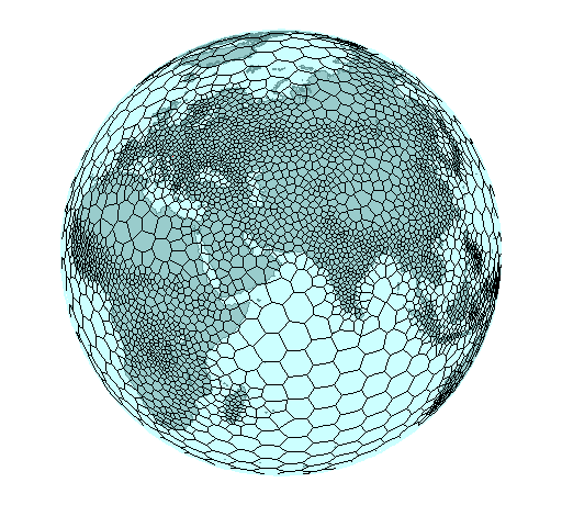
By contrast, the partitioning scheme used in the Hipparchus model is based on spheroidal cells analogous to planar Voronoi polygons. The definition of the structure is simple. Given a set of distinct (center)points, a spheroidal polygon-cell corresponding to one of them is defined as a set of all surface points "closer" to it than to any other member of the centerpoint set. For each surface point, the minimum "distance" to any point in the set of centers can be determined: if there is only one centerpoint at such a distance, the point is within a cell. If there are two, it belongs to an edge. If there are three, the point is a vertex. A dual of the set of polygons is obtained by connecting the centerpoints which share an edge.
The application can define a pattern of cells by any purposefully distributed set of centerpoints. Since these are defined by their normals, the partitioning scheme is completely free from condescending to any numerically singular surface point. The distribution of centerpoints can be based on any combination of criteria selected by the application: data volume distribution, system activity patterns, maximum or minimum cell size limits. It can even represent an existing set of spatial framework items, e.g. geodetic control stations.
A sort-like algorithm produces the digital model of the dual. The cell frame structure is thus reduced to a list of global, ellipsoid coordinates of centerpoints and a circular list of neighbor identifiers for each cell. If the application requires that a limit be placed on the maximum "distance" between neighboring centerpoints, the algorithm must be capable of bridging the "voids", and null items must be recognizable in the circular list. This data structure is used extensively by all spatial algorithms. Unlike systems in which location of the cell is implied in its identifier, the Hipparchus model requires explicit recording of the global coordinates of cell centers. Method of storage and access to this data can therefore have considerable influence on the efficiency of spatial processing.
A cell is assigned an internal coordinate system with the origin at its centerpoint. As mentioned before, the mapping function between global and cell systems is an ellipsoid-modified stereographic projection. The "transformation algorithms" (in both directions) consist therefore of nothing but a few floating-point multiplications.
"Finite Element Cartography". If a large volume of data has to be transformed into output device coordinates based on a specific conventional cartographic projection, only a few points on the cell (or the display surface) frame will have to be transformed using a rigorous cartographic projection calculation. Based on the frame data/display correspondence, parameters of a simple polynomial transformation are easily calculated. Volume transformations will again require only a few multiplications, and can be set to produce the result directly in hardware coordinates of an output device. This type of manipulation can be of particular value if a complex geometronical function has to be applied over the complete surface of a dense data set, for instance in transient cartographic restitution of digital remote sensor image material.
One of the most often executed algorithms in the model will probably be the search for the "home cell" of an arbitrary global location. Selection of the first candidate cell is left to the application, in order to exploit any systematic bias in either transient or permanent location reference distribution. A list of all neighbors is traversed, and distances from the given location to the neighbor centerpoints are determined. If all these distances are greater than the distance from the current candidate centerpoint, the problem is solved. Otherwise, the minimum value indicates a better candidate. While the algorithm is very straightforward, its efficiency will be extremely sensitive to the selection of the spheroid "distance" definition and numerical characteristics of global coordinates. The same will apply to most combined list-processing and numerical algorithms employed by the model.
While Voronoi polygons have often been used in computer algorithms solving various classes of planar navigation problems, at the time of this writing no record was found of the use of an equivalent global, spheroidal structure as a partitioning scheme in a geometronical computer system.
Points: Digital representation of a point data element is simple: it consists of a cell identifier and local (cell) coordinates. Even with fairly large cells, the global-to-local scaling will ensure equivalent spatial resolution in case where local coordinate values have only one-half of the significant digits used for global coordinate values. Since the efficiency of external storage use and the associated speed of I/O transfer can be of extreme importance in a large database, the following numerical data are of interest:
If a 64-bit global, a 32-bit local coordinate values and 16-bit cell identifier are used, the volume data point representation will require only 80 bits, and will still yield sub-millimeter resolution. 80 binary digits are capable of storing 2**80 (approximately 1.2E24) distinct values; the surface of the Earth is approximately 5.1E20 square millimeters. The ratio of these two numbers (approximately 69 out of 80) represents the theoretical memory utilization factor; practically, the margin allows significant variation in cell size and use of various computational conveniences (floating point notation, cell range encoding, e.t.c.). This utilization factor compares to 69 bits out of 128 if the point is represented by latitude/longitude in radian measure, and 69 out of 144 bits (typically) if a conventional, wide-coverage cartographic projection system plane identifier and coordinates are used. Furthermore, various external storage compression schemes that take advantage of the re-occurring cell identifier are likely to be significantly simpler and more effective than any compression scheme of a pure numerical coordinate value.
It is important to note that in Hipparchus model cell coordinates of a point are not used for a numerical solution of metric problems; their purpose is to provide a compressed coordinate storage format for high-volume data, and to facilitate generation of the transient, analog view of the data.
Lines: One-dimensional objects are represented by an ordered list of cells traversed by the line, and - within each cell - a list, (possibly null) of vertices in the point format described above. If the application requires frequent evaluations of spatial unions and intersections, it might be efficient to find and store permanently all points where lines cross cell boundaries. Their internal representation (permanent or transient) is somewhat modified in order to restrict their domain to the one-dimensional edge, but their resolution and storage requirements will be comparable to the general point format used by the model.
Regions: Two-dimensional objects are represented by a directed circular boundary line and an encoded aggregate list of cells that are completely within the region. When compared to simple boundary line circular vertex list, this structure makes the evaluation of spatial relationships significantly more efficient. The solution will often be reached by simple manipulation of cell identifier lists, instead of the evaluation of boundary geometry. The number of cases where, ceteris paribus, this will be possible, will be inversely proportional to the average cell size. (In example in Fig. 3, boundary geometry examination will be confined to three cells.) This representation of a two-dimensional object is a combination of the traditional boundary representation and schemes based on regular planar tessellations. It offers the high resolution and precision usually associated with the former, while approaching the efficiency of relational evaluations of the latter. In addition, it does not violate the true spherical nature of the data domain. For instance, if [A] is a region, then NOT [A] is an infinite, numerically ill-defined region in a plane. By contrast, on any spheroidal surface NOT [A] is the simple finite complement.
Orbit Dynamics: Practice abounds with examples of problems encountered in attempts to integrate remote sensing and existing terrestrial data. Even in instances where the spatial geometry can be defined with sufficient precision, it is common to cast (by "pre-processing") the digital image produced by a satellite sensor into a specific plane projection system and pixel aspect ratio and orientation. This unnecessarily increases the entropy of remotely sensed data available to applications requiring different or no planar castings. In many instances, problems will disappear if the application is given the ability to manipulate the original, undistorted, observation geometry.
A general-purpose geopositioning software tool must therefore provide efficient evaluation of basic time/geometry relationships within the orbital plane, and the ability to transfer the locations from an instantaneous orbit plane to its primary frame of spatial reference. (More complex calculations are probably application-specific and are restricted to infrequent adjustments of orbit parameters.)
The geometry functions described already suffice to define any orbit at the convenient epoch - e.g. the time of the last parameter adjustment. To find a position (in the orbital plane) of a platform at a given time, a direct solution of the problem postulated by Kepler's second law is required. (Same as in geodetic problems mentioned previously, this "direct" problem requires an iteration, while the "inverse" yields a closed solution.) Any increase of orbit eccentricity will affect the number of iterations, but the same software component can be used to solve both near-circular and steep orbits. Common 64-bit floating point representation will preserve millimetric resolution even for geosynchronous orbits. Rigorous modelling of general precession can be achieved simply by an additional vector rotation about the polar axis. This is combined easily with sidereal rotation, required in any case for transfer of position between the inertial and terrestrial frames of reference.
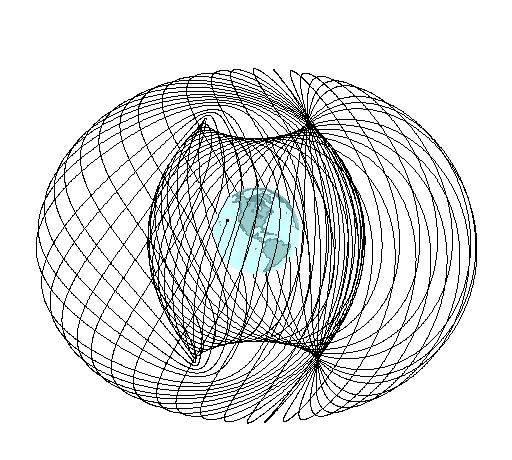
Fig. 4: Orthographic view of a precessing orbit
Use of computers in mapping is as old as the computer itself: the first commercially marketed computer, UNIVAC 1, was used in 1952 to calculate Gauss-Krueger projection tables. With the development of computer graphics, it quickly became common to store and update a graphical scheme representing a map. Until very recently, the main object of this process remained the production of graphical output that was not substantially different from a conventional analog map. While the production of the map was thus computerized, the ability of an "end-use" quantitative discipline to employ a computer to solve complex spatial problems was not addressed. The use of a "computer map" was precisely the same as that of a traditional, manually produced document.
All quantitative disciplines are facing the same demands as cartography to increase precision, volume and complexity of data which can be efficiently processed. Hence, computer applications in those disciplines require "maps" from which spatial inferences can be derived not only by the traditional map user, but also by a set of computer application programs. To a limited extent only, this has been achieved in applications which could tolerate severe limitations on area of coverage, data volumes, or spatial resolution requirements. Location attributes in these computer systems are usually based on an extended coverage ellipsoid-to-plane conformal projection: a numerical model developed for a completely different purpose.
Computer systems requiring extensive spatial modelling combined with high resolution and global coverage need powerful yet efficient numerical georeferencing models. It is unlikely that these can be based on conventional cartographic techniques. Numerical methodologies designed specifically for the computerized handling of spatial data have the best potential for providing generalized solutions.