A Seamless Global Terrain Model in the Hipparchus System
Hrvoje Lukatela,
Geodyssey Limited
http://www.geodyssey.com/
Paper presented at the International Conference on Discrete Global Grids,
Santa Barbara, 26 - 28 March 2000
Abstract
This paper outlines the steps used to construct seamless global
triangular networks similar to the planar TIN commonly used to
facilitate terrain modeling and volumetrics. It is based on global
coordinates and a planetary surface tessellation using spheroidal
Voronoi polygons. The techniques used to extend the surface modeling
across the Voronoi cell boundaries are presented. The paper also outlines
the strategy used for the efficient retrieval of only those parts of the
model that are visible in a transient view, as well as the platform- and
projection-independent approach to surface rendering.
Introduction
 Representation of the physical surface of the Earth in digital
systems is a subject of considerable current attention. As the area of
the coverage of such systems increases, it becomes necessary to provide
methods to model very large, continuous surface conglomerates in a manner
which does not violate the surface integrity (i.e., which does not impose
hard partitioning as an artifact of the digital model), but, at the same
time, provides an efficient spatial index to a small section of the surface
of transient interest.
Representation of the physical surface of the Earth in digital
systems is a subject of considerable current attention. As the area of
the coverage of such systems increases, it becomes necessary to provide
methods to model very large, continuous surface conglomerates in a manner
which does not violate the surface integrity (i.e., which does not impose
hard partitioning as an artifact of the digital model), but, at the same
time, provides an efficient spatial index to a small section of the surface
of transient interest.
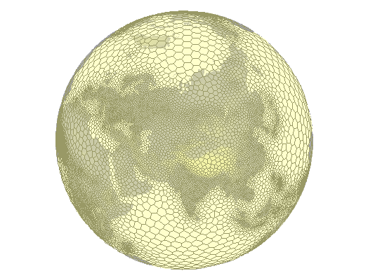
Figure 1: A "global grid" of Voronoi polygons
The Hipparchus Geopositioning Model
(outlined in considerable detail in a web-resident publication titled:
Hipparchus Geopositioning Model: an Overview)
provides a method of construction and manipulation of geometric objects
of various levels of complexity (points, lines, areas and surfaces)
in a manner which imposes no restrictions on their spatial size or
shape. The system is based on two major computational geometry constructs:
use of the vector components of the ellipsoid normal instead of the latitude
and longitude angles and data-density driven tessellation of the planetary
surface using a global grid of spheroidal Voronoi polygons.
The position of a point on the surface of the ellipsoid is best given
by a numerical definition of the normal to the surface at that point.
The common global coordinates - latitude and longitude - are angles:
the first of the two is between the normal and the Equatorial plane
and the second between the Equatorial plane projections of the normal and
the projection of the prime meridian. Traditional geodetic computations
(for instance: given are two known points, determine the length and the
azimuth of the shortest line that connects them...) are based on
trigonometric functions of those angles and on the expansion of the power
series of the eccentricity of the ellipsoid. The angles, however, present
two problems when used for computations on digital computers: transcendental
functions (sines, cosines) require many more CPU cycles than the algebraic
primitives (addition, multiplication) and their areas of singularity must
be compensated with complicated and error-prone code. Thus replacing angles
with vector components of the ellipsoid normal was noticed as potentially
beneficial as soon as the digital computers were incorporated into the
geodetic practice (cf. Bomford (1975), remark on formulae "symmetrical and
better for computation...", p. 593 - under 'Cartesian Coordinates in
Three Dimensions'). Hipparchus computations are consistently based on
the ellipsoid normal given by its vector components instead of the latitude
and longitude angles.
A "global grid" is, in the most general sense, a geometrical subdivision
of the planetary surface which assists in the organization (partitioning,
indexing, etc.) of globally-distributed digital data. "Regularity" of
the grid usually translates to simple data structures and straightforward
classification algorithms. Since no regular and isometric tessellation of
the sphere (beyond five platonic solids) is possible, practical applications
have two alternatives: to retain in the design of the "grid" as much
"regularity" as possible, to be rewarded with a considerable algorithmic
elegance, but at the expense of the ability to perform fast and accurate
geodetic computations (see Dutton, (1999) for a well-known example of such
approach), or to accept the "irregular" nature of the grid while attempting
to make computations based on it as fast and as precise as possible.
The Hipparchus system makes no attempt to produce a "regular" grid. Instead, the
grid is designed so that any particular implementation of the grid can match
the density of the data that inhabits it and so that the parameters which
numerically define the grid "cells" assist (and not hinder) the speed and
precision of geodetic computations and spatial algebra productions.
(Figure 1 shows a sample of such grid with the density derived from the
density of the human population). It is based on the surface subdivision
known as "Voronoi polygons": a purposefully selected finite and discrete
set of "cell-center" points subdivides the surface so that any surface point
is uniquely associated (i.e., it "belongs to") the member of the set that
it is closest to. The point classification is accomplished using only
distance calculations. Point, line, area and surface object sets are in
turn defined in terms of the cells they occupy and the vertex coordinates,
represented not by a the full (global) vector representation of the
ellipsoid normals, but by the vector difference from their respective
cell center points. An extended introduction to and computational geometry
treatment of the Voronoi polygons can be found in O'Rourke (1994).
This paper outlines the canonical representation of the surface object,
and explores the techniques which are used to operate upon it.
While the context and the examples used in this paper center on the
representation of the terrain, such objects can be used to represent
any continuous function for which a sufficiently dense set of point-location
dependent scalar values are known, and about which we know enough to
postulate that each planetary surface point will have one (and only one)
measured or interpolated function value.
Triangulated Irregular Network - TIN
 The triangulated irregular network (TIN) is an often used surface
representation method in planar computational geometry. Description of TIN
data structures and the algorithms (including C language source code)
can be found in both Ambroziak (1993) and Lischinski (1994). The TIN
approximates a continuous surface with a mesh of triangles which
more or less coincide with it. The quality of this approximation depends
on the combination of the method by which the elevation measurement
points have been selected, and the triangulation strategy.
The implementation described herein assumes a more-or-less uniform
density of significant points and starts with a simple "least-diagonals"
fast iterative planar triangulation algorithm. It is open to accept
different triangulation strategies - presumably matching more closely
the peculiarities of the input data generation process.
The triangulated irregular network (TIN) is an often used surface
representation method in planar computational geometry. Description of TIN
data structures and the algorithms (including C language source code)
can be found in both Ambroziak (1993) and Lischinski (1994). The TIN
approximates a continuous surface with a mesh of triangles which
more or less coincide with it. The quality of this approximation depends
on the combination of the method by which the elevation measurement
points have been selected, and the triangulation strategy.
The implementation described herein assumes a more-or-less uniform
density of significant points and starts with a simple "least-diagonals"
fast iterative planar triangulation algorithm. It is open to accept
different triangulation strategies - presumably matching more closely
the peculiarities of the input data generation process.
The data structure used to represent a planar TIN is simple and
shows only minor variations from one implementation to another.
It consists conceptually of an array of points and an array of
triangles. The two may be doubly linked, but commonly only
the triangles are linked to their vertices. Additionally, each
triangle is linked to its three neighbors, with a flag value
to signal that a triangle edge is at the same time the edge of the
TIN (i.e., it is an "outside" edge). Most triangulation algorithms
produce a structure in which all outer edges form a planar convex hull.
A point array element consists of planar coordinates and elevation.
If the shading or perspective rendering is anticipated, triangle
normals might be included in the data; this however would be worthwhile
only if the cost of re-computing the triangle orientation far outweighs
the cost of additional storage and, usually of even greater significance,
the time required to access it.
The main difficulty in the implementation of computational geometry
algorithms usually stems from the need to properly predict all (or at
least all likely) degeneracy and singularity cases. (See in particular
comments under "Robustness" in Lischinski (1994)). While the implementation
described in this paper is no exception, it is interesting to note that
all such problems were encountered (and hopefully resolved) in the planar
("in-cell") geometry domain.
A TIN in a Global Voronoi Grid
 In general, the Voronoi polygon grid used to model the TIN will be used
to provide the spatial framework for a number of other object classes.
The only requirement that the implementation of TIN data will place on the
grid is that the density of the elevation points remains approximately an
order of magnitude above the density of the Voronoi polygon centers.
In this - and a number of other characteristics - a TIN object in a global
Voronoi grid parallels the combined characteristics of Hipparchus point
and line sets. This TIN will additionally consist simultaneously of two
levels of triangle/elevation data: high-volume triangles with source data
points as their vertices and low-volume, large triangles with cell-center
and end-points of cell edges as their vertices.
In general, the Voronoi polygon grid used to model the TIN will be used
to provide the spatial framework for a number of other object classes.
The only requirement that the implementation of TIN data will place on the
grid is that the density of the elevation points remains approximately an
order of magnitude above the density of the Voronoi polygon centers.
In this - and a number of other characteristics - a TIN object in a global
Voronoi grid parallels the combined characteristics of Hipparchus point
and line sets. This TIN will additionally consist simultaneously of two
levels of triangle/elevation data: high-volume triangles with source data
points as their vertices and low-volume, large triangles with cell-center
and end-points of cell edges as their vertices.
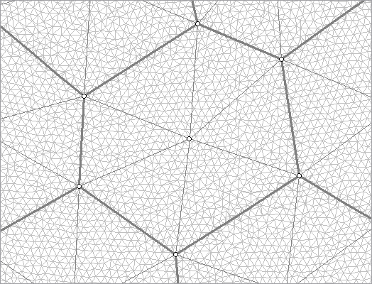
Figure 2: TIN in a Voronoi grid
The source data used in a construction of the Hipparchus TIN object
is a Hipparchus point set with elevations. The construction algorithm
proceeds cell by cell, transferring the point coordinate and elevation
data from the point set into a two-level TIN structure consisting of
both individual triangles and the values that describe the elevation
of cell-sector triangular vertices. In each cell, the process starts
with a selection of all those points that are inside the cell and those
points in the neighbor cells that fall within some distance of the
shared edge. A triangular grid produced in this step is then intersected
with the cell boundary. All triangle edge/cell edge intersection points
are assigned an interpolated elevation and marked as "points on the hull".
(This can be done, since the Voronoi polygon is at the same time a convex
hull of all points in its interior). These points are kept in the final
surface representation. Description of planar convex hull and algorithms
used to construct it can be found in Sedgwick (1983).
A second triangulation (that includes only cell interior and cell-edge
points) follows, this time as a faster, "forced hull" process.
The triangles of this second triangulation are stored - together
with the point coordinate and elevation data - in a final cell-oriented
series of structures representing the surface. Similar to other Hipparchus
objects, it is a hierarchical set of tables, at the center of which is
a table of "cell headers". It describes that part of the surface which is
"over" the cell, and its most important elements are:
- Cell identifier
- Coordinate array pointer and count
- Count of the cell interior points in the above
- Triangle array pointer and count
- Triangle neighbors array pointer and count
- Minimum, maximum and mean cell elevations
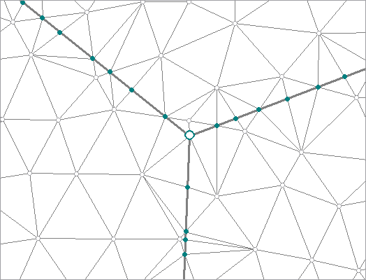
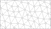
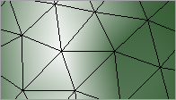
Figure 3: Different types of elevation points
The final TIN point array contains three types of points (clearly
distinguished in Figure 3), in order-of-magnitude decreasing numbers:
- Elevation points transferred from the source point set.
- Cell/triangle edge intersections with linearly interpolated elevations.
- Cell vertex points with spatially interpolated elevations.
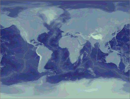
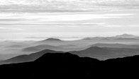
Figure 4: Hypsographic rendering of a global TIN
The test data set (see Figure 4 for its hypsographic representation)
used to produce the illustrations of this paper, has been derived from a
5-minute gridded set of elevation points, and used extensively in the
development and code testing. A high density Voronoi grid was used as
a sampling framework, to avoid an artificially high
(and meaningless) data density in high latitudes, and to reduce
the point count to a level commensurate with the overall quality of
the elevation data. The result of this process was a Hipparchus point
set with about 200K points covering the planet in a generally uniform
pattern. In addition to its use in the testing, it is anticipated that
it will also be used to complete the planetary surface coverage for
local (regional, continental, etc.) elevation data sets available in
higher density and precision. This strategy is not unlike the frequent
use of a Hipparchus Voronoi index center-point set called "isotype",
which provides a similar function for regionally-biased grids.
The size of the disk files is approximately 2.5 MB for the source point
set, and approximately 8.4 MB as a TIN. In the current implementation,
all in-cell triangle indices are 32-bit integers; this removes any
practical restriction on the number of triangles in a single cell.
Elevations are recorded as 32-bit floating point numbers.
TIN Rendering
 TIN rendering is implemented in a series of functions that belong to
the general section of the Hipparchus Library dealing with "geographics".
A TIN can be rendered in a "reduced dimensionality" mode, to generate
only the points and lines (triangle edges) without the full surface
representation. This mode was used to generate Figure 3. The Figure and
the other illustrations in this paper were created using a scripted
geographical workbench program called GALILEO, available for free download
from Geodyssey's web page at
http://www.geodyssey.com/.
TIN rendering is implemented in a series of functions that belong to
the general section of the Hipparchus Library dealing with "geographics".
A TIN can be rendered in a "reduced dimensionality" mode, to generate
only the points and lines (triangle edges) without the full surface
representation. This mode was used to generate Figure 3. The Figure and
the other illustrations in this paper were created using a scripted
geographical workbench program called GALILEO, available for free download
from Geodyssey's web page at
http://www.geodyssey.com/.
In cartographic applications a TIN is most often rendered as one of the two
graphical artifacts: a hypsographic scale color fill or a shaded surface.
The first assigns to each pixel a color dependent on the point elevation,
the second assigns a color dependent on the spatial orientation (slope and
azimuth) of the surface. Figures 5 and 6 illustrate the difference: both
show the map background-fill "layer" generated from a global TIN for an area of
the European Alps. Hydrographic network and political boundaries are also shown;
both are expected to be - to some extent at least - in an easily verifiable
relationship to the surface elevations.
Of the two, hypsographic scale color fill is more demanding of the graphical
programming, as it requires painting of pixels that belong to a single triangle
with a range of colors. (As opposed to shading, where all the pixels that
represent one triangle are in general of the same color). We will therefore
in the following concentrate on the hypsographic scale TIN rendering.
The central computation geometry process used in this type of rendering is the
ubiquitous triangle "gradient fill": given the x and y (image) coordinates of
three vertices and their associated "z" value, fill all pixels "inside" the
triangle with a color value commensurate to the interpolated value of "z".
This interpolated value is a value that a respective point of the plane
defined by three points (vertices) would have.
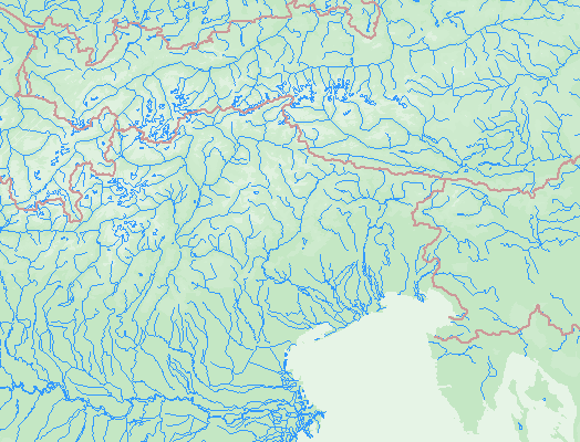
Figure: 5 Hypsographyc rendering
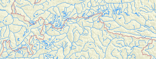
Figure: 6 Shaded rendering
Because of the multiplicity of environments in which this type of
rendering is performed, there are different levels at which the
division of labor between the application code (including any libraries
used), the graphical platform and - possibly - the display hardware
can take place. For the Hipparchus Library, we assumed there are at least
three such levels, and so provided the means to allocate control to a
lower level component (i.e., either the graphical platform or the
hardware) at any of those three levels. Their application program
interface can be described by the dimension, as follows:
- Point
- A single pixel is set to a color of the invoker's choice.
- Line
- Pixels of a scan-line segment with a given y and two end-point
x coordinates are set to a linear gradient of colors linearly
interpolated between given end-point color values.
- Area
- All pixels inside a triangle are filled with colors interpolated
between the given color values of the vertices.
The first level is available in even the most basic graphical application
development environments; the last one is implemented in most
"2-D accelerated" graphical device drivers and is supported in
graphical platforms targeting such devices. Thus an application rendering
a TIN would keep invoking Hipparchus Library functions to the
point-level under the Win32 API, and pass a whole triangle to an Open GL API.
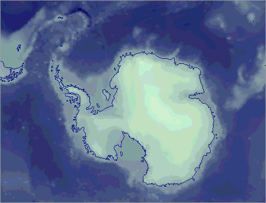
Figure: 7 Sample surface, rendered in (relatively) large scale
A high-latitude section of the global TIN depicted in Figure 7
illustrates another unique advantage of the TIN representation in a
Voronoi grid. As mentioned before, all vertices on the cell edge will
have an interpolated elevation assigned to them. Likewise, a mean
elevation value for the whole cell is a natural by-product of the TIN
construction process. This data (cell mean and edges values) can be
used as a "generalized" representation of the same TIN: it consists
of a set of cell-segment level triangles, probably an order of magnitude
fewer per given area than the original TIN. (cf. outlined points and
large triangles formed by them in Figure 2). When the scale of rendering
becomes sufficiently small, the application can choose to render only
the large triangles, thus decreasing the rendering time considerably.
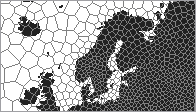
Applications will often store Hipparchus Binary Objects (on disk or in
a database) so that the low-volume cell-related values are separated
from the high-volume point coordinates. If this is the case, rendering
based only on the cell-level values (such as depicted on the small-scale
map in Figure 8) will require at least an order of magnitude fewer disk
transfers than the rendering of Figure 7 - despite the fact that both
are generated from the same surface object.
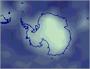
Figure 8: Cell-level generalization
Conclusion
A TIN as a Hipparchus Binary Object shares many architectural similarities
with point sets, line sets and regions constructed and recorded in the
context of global Voronoi grids. Its construction is based on a planar
triangulation within the cell boundaries. Triangle information storage
follows the common planar TIN model, but an additional set of elevations
is stored to represent the cell edge elevation profile. Simple,
straightforward and conjugate linear interpolation of elevations on the
edge guarantees that no artifact will be introduced at the cell edge.
The cell-based data structure representing the whole TIN provides a
simple and fast determination of the elevation at an arbitrary selected
surface point, and triangle rendering fits well with the API of common
graphical platforms. A novel approach to the problem of generalized
rendering is another benefit of the Voronoi grid.
References
-
Ambroziak, R.A., Cook C.A., Woodwell, G.R. and Wicks R.E.:
Data, Software, and Applications for Education and Research in Geology
(CD publication), United States Geological Survey Open File Report 93-231, 1993.
-
Bomford, G. Geodesy, London, Oxford University Press, 1975 ed.
-
Dutton, G. H.:A Hierarchical Coordinate System for Geoprocessing and Cartography,
Springer Lecture Notes in Earth Sciences 1999.
-
Lischinski, D.:Incremental Delauny Triangulation, article published in
The Graphics Gems Series, Volume IV, pp. 47-59, AP Professional 1994.
-
O'Rourke, R.:Computational Geometry in C, Cambridge University Press 1994.
-
Sedgewick, R.:Algorithms, Addison-Wesley 1983.
...