Ellipsoidal Area Computations of Large Terrestrial Objects
Hrvoje Lukatela,
Geodyssey Limited
http://www.geodyssey.com/
Paper presented at the International Conference on Discrete Global Grids,
Santa Barbara, 26 - 28 March 2000
Abstract
The mathematics of area computation on the ellipsoidal planetary
surface is straightforward; it is however rarely implemented in
its rigorous form. Most spatial information systems dealing with
two dimensional objects treat the area not as a simple derivative
of the object definition geometry, but rather as an artifact of
its representation in a particular planar representation. This
approach fails when no single, canonical planar representation is
either practical or desirable, or when the spatial extent of the
object exceeds the useful coverage of a single planar projection.
The Hipparchus geopositioning model represents two dimensional
terrestrial objects in the context of an irregular global grid
consisting of spheroidal Voronoi polygons. This paper presents
the strategy and outlines the implementation of area computation
for such objects. It assumes that efficiency is as important as
is the precision, and that the objects can be of any size, shape
and topological complexity. The speed and accuracy of the
computation is examined by applying it to a large, global object
of high data volume and considerable topological complexity.
Introduction
 This paper presents a particular numerical solution to a rather
straightforward and well-defined mathematical problem: given a
two-dimensional object of an arbitrary complex topology on a surface
of an ellipsoid of rotation, find its area. Several elements of the
underlining mathematics are worth noting at the outset:
This paper presents a particular numerical solution to a rather
straightforward and well-defined mathematical problem: given a
two-dimensional object of an arbitrary complex topology on a surface
of an ellipsoid of rotation, find its area. Several elements of the
underlining mathematics are worth noting at the outset:
-
The total surface of an ellipsoid of rotation can be expressed as
a closed (but transcendental) function of its semi-minor and
semi-major axes.
-
The area of a pseudo-trapezoidal figure bounded by two meridians
and two parallels leads to a single ellipsoidal integral over the
latitude domain.
-
The area of a triangle - with geodesics as its sides - leads to
a double ellipsoidal integral over the geodesic lengths.
Even the mathematically simpler - trapezoidal - decomposition
results in an integral that requires a binomial series expansion.
In addition, the substitution of the continuously changing width of
latitude-bands for a figure bounded by a geodesic leads to an
approximation, the magnitude of which depends on both the band height
and the local azimuth of the geodesic. The decomposition into triangles
results in a similar, but even more complicated numerical solution.
In either case, the decomposition of topologically "deep" two
dimensional objects into either pseudo-trapezoidal or triangular
components can lead to rather complex implementation problems.
A good overview of the ellipsoidal geometry and the algebra
and calculus used to implement common geodetic computations can
be found in either Jordan (1958) or Bomford (1975).
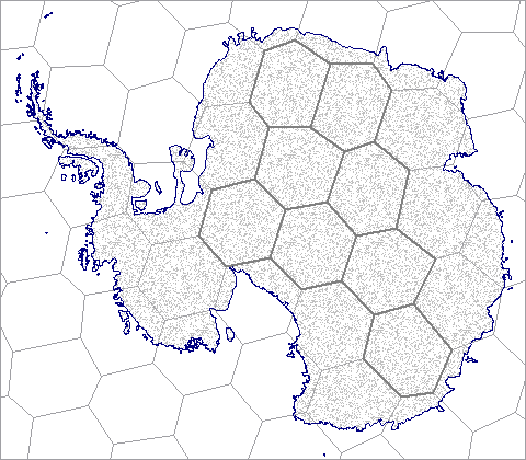
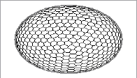
Figure 1: A two-dimensional object in a spheroidal Voronoi grid
If the two-dimensional ellipsoidal surface object is already
represented in a form which provides a convenient basis for the
geometrical decomposition, it will be advantageous to use such
representation as a basis for the area computation. This is the
case in the Hipparchus Geopositioning Model, where an object is
represented in an irregular global grid of Voronoi polygons.
(The full presentation of this model is outlined in a web-resident
publication titled:
Hipparchus Geopositioning Model: an Overview). It is an
example of a "constructive index", where the object geometrical
integrity remains intact, and the infrastructure required to
access parts of the object that belong to one index block
(data cell, tile... etc.) exists "in addition" to the data
defining its geometry. Figure 1 depicts an object in a global
Voronoi grid. We will - later on in this text - recapitulate
those features of this type of object representation which
influence directly the area computation. For now, we note only
that there are some cells ("boundary cells") through which the
object boundary "meanders" and some cells ("interior cells")
which are completely encompassed by the object. The area of an
object will be determined by summing up the area of all interior
cells and adding to this the partial area - that portion covered
by the object - of all of its boundary cells.
Area of Ellipsoidal Voronoi Cells
 We will first outline the method for determining the area of any
Voronoi cell. This is done by subdividing the cell into triangles
with neighbor edges as a base and cell center as the opposite
vertex. The edges of these triangles are segments of great
circles on a sphere related to the ellipsoid (on which both the
object boundary and cell-center coordinates are defined by their
geodetic coordinates) by conformal ellipsoid to sphere mapping.
While these edges are not ellipsoidal geodesics, the maximum line
displacement is both relatively small (2.5 meters for a line similar
to the one discussed below in the context of UTM mapping) and the
"gain" and "loss" tend to be of the same magnitude when all the edges
along the cell boundary are considered. The area of these triangles
is then computed by spherical productions, but using a constantly
changing radius determined by the mean curvature of the ellipsoid
surface in the cell center.
We will first outline the method for determining the area of any
Voronoi cell. This is done by subdividing the cell into triangles
with neighbor edges as a base and cell center as the opposite
vertex. The edges of these triangles are segments of great
circles on a sphere related to the ellipsoid (on which both the
object boundary and cell-center coordinates are defined by their
geodetic coordinates) by conformal ellipsoid to sphere mapping.
While these edges are not ellipsoidal geodesics, the maximum line
displacement is both relatively small (2.5 meters for a line similar
to the one discussed below in the context of UTM mapping) and the
"gain" and "loss" tend to be of the same magnitude when all the edges
along the cell boundary are considered. The area of these triangles
is then computed by spherical productions, but using a constantly
changing radius determined by the mean curvature of the ellipsoid
surface in the cell center.
The method presented here shares two salient principles with the one
devised by Tobler and Kimerling, as described in Kimerling (1984):
the first is the use of local ellipsoidal radii in spherical triangle
area productions and the second is the tracking of positive and
negative area contributions based on the direction of the boundary
segment. The latter parallels the procedural makeup of the planar
polygon area computation and provides an effective way to keep the
non-numerical programming complication within reason, while at the
same time avoiding any restriction on the level of the topological
complexity of the objects for which the area is calculated.
In geodetic computations, the expression for the mean radius of
the ellipsoid surface in a given point is commonly referred to as
Gauss' formula: r = sqrt(m*n)
(where m and n are radii of the meridian
and prime vertical, respectively). The conventional computation of
the mean radius uses the ellipsoidal eccentricity term - an
unnecessary complication in computation on digital computers.
The preferred method uses tsq: a latitude
(phi) dependent square of the free term of the tangential
plane, defined directly as a function of the sine and cosine of the
point of tangency and the major and minor ellipsoid semi-axes
(a and b respectively), as follows:
s = sin(phi)

c = cos(phi)

tsq = a*a*c*c + b*b*s*s

r = (a*a*b)/tsq
This method of mean ellipsoid radius computation is especially
convenient for systems such as Hipparchus, which represent the
location of a point using the direction cosines of its ellipsoid
normal: the evaluations of s and c require
no expensive transcendental computations. Also, the tsq term finds a
repeated use in many different ellipsoid geometry propositions.
No a priori error term has been derived for this "finite element"
ellipsoid-to-sphere approximation; the total area of all cells so
computed can however be compared (and adjusted) to the total
ellipsoid surface. (See below, under "Some Numerical Results",
for details). Since we assume that a system will be required to
produce the area of many different objects, represented in the
context of the same global grid, an array of areas - one element
for each cell - will be conveniently stored with the
other data in the structures representing the Voronoi polygons.
Computing the area of a spherical triangle for which the lengths of
all three sides (a, b and c) are given can be
done using two different approaches: by applying Legendre's
approximation, or by L'Huilere's theorem. The former states that
the area of a spherical triangle will be getting closer to the area
of a planar triangle with the same side lengths, as the ratio of the
triangle perimeter divided by the spherical radius gets smaller.
The latter is, on the other hand, a rigorous evaluation of the
spherical triangle area in terms of the three sides. To compare the two:
P = sqrt(s*(s-a)*(s-b)*(s-c))
versus:
P = 4*atan(sqrt(tan(s/2)*tan((s-a)/2)*tan((s-b)/2)*tan((s-c)/2)))
(where s is the common shorthand notation for the
half-sum of all three sides)
Implementations which impose a low maximum cell radius limit might
take advantage of a considerably faster Legendre's approximation.
The implementation used to derive the numerical examples given below
is, however, based on the second (L'Huilere's) expression, applied to a
"local" sphere with the radius equal to the mean ellipsoid radius at
the cell center.
Area Computation in Boundary Cells
 The determination of the area of an object in a boundary cell
requires no additional mathematics. If an object is topologically
well-defined, its area inside a boundary cell will consist of a
finite number of distinct "faces", each bounded by a closed ring.
The ring may consist of either the segments that all belong to
the object boundary, or, in the general case, a combination of object
boundary and cell edge segments. In a procedure directly
paralleling the usual implementation of planar polygon area
computation, we can traverse the ring, and accumulate triangular
areas subtended from each segment and the coordinate origin -
adding or subtracting, depending on the radial direction of
the boundary segment respective to the coordinate origin.
The determination of the area of an object in a boundary cell
requires no additional mathematics. If an object is topologically
well-defined, its area inside a boundary cell will consist of a
finite number of distinct "faces", each bounded by a closed ring.
The ring may consist of either the segments that all belong to
the object boundary, or, in the general case, a combination of object
boundary and cell edge segments. In a procedure directly
paralleling the usual implementation of planar polygon area
computation, we can traverse the ring, and accumulate triangular
areas subtended from each segment and the coordinate origin -
adding or subtracting, depending on the radial direction of
the boundary segment respective to the coordinate origin.
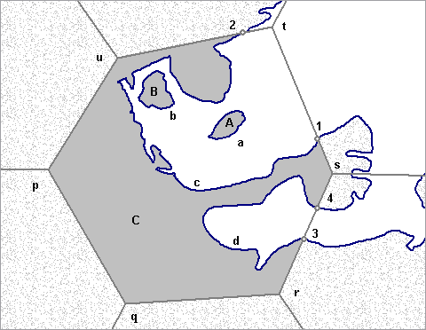
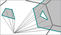
Figure 2: Geometry of a boundary cell
We will next identify some area computation pertinent features
of the object geometry definition in an example of a boundary cell,
as depicted in Figure 2. (It is an enlarged part of the object shown
in Figure 1). The topological decomposition of the object presented
in the following is essentially the same as it would be if the
object was a planar one - thus additional details, definitions and
code segments can be found in many sources describing planar
computational geometry - for instance Bowyer (1983).
The fundamental geometrical element is a "fragment":
an ordered array of vertices forming the object boundary, in
either a closed ring, or starting and ending on the cell boundary.
There are four boundary fragments in the example: a, b,
c and d; two of them are closed rings (a and
b), and two are connecting cell boundary crossing points
(fragment c, connecting crossing points 1 and 2;
and fragment d, connecting points 3 and 4).
For each fragment, we note that the start point is the point where
the object boundary "enters" the cell, and the fragment end point is
the point where the boundary "exits" the cell.
Fragments are directed in the mathematically positive sense, such that
the object interior is always on the left-hand side of the boundary
line. This ensures that the "voids" will produce a negative
contribution to the total area, regardless of how "deeply nested"
the topology of the object is.
One or more fragments form the boundary of a "face" - a single
continuous, connected area. In the example, there are three faces:
A, B and C. Faces A and B are
formed by single ring fragments a and b. Face C
is formed by fragments c and d. In addition to the two
fragments, the boundary of face C also requires two cell-edge
line segments: first one from the end point of the fragment d,
to the cell vertex s, to the start point of the fragment
c and the second, from the end point of fragment c,
through the cell vertices u, p, q and r,
to the start point of the fragment d.
A canonical representation of the Hipparchus system two-dimensional
objects identifies only the distinct boundary fragments, and not
the faces they form. No spatial algebra proposition
(e.g., "polygon overlay") requires this knowledge, and all such
propositions would thus be burdened with the additional code if
required to keep track of the fragment/face relationship.
The area computation algorithm must therefore "construct" the
faces as and when required. This information is used implicitly,
in the ring traverse order, and is not stored permanently.
This "construction" is trivial for faces which are formed by a
single closed fragment (A, B); and somewhat involved
for the faces (C) that are composed of both object and cell
boundary.
The computation of an object area in a boundary cell consists of
two phases. The first one is a simple traverse of all fragments.
Closed fragments present no special problem: their area
contribution is accumulated as they are encountered.
For open fragments (i.e., those that start and end on the cell
boundary) both boundary crossing points are stored in a table,
which lists the point type (start or end), fragment identification
(in form of a pointer), cell neighbor index of the crossing
point, and the distance from the closest "upstream" cell vertex.
If the cell across the p-q edge is the first
(index 0) neighbor in the (circular) list of cell neighbor
cells, then for fragment c two entries are stored in the
table: one for entry point 1, with neighbor index 3
and s-1 distance; and another for exit point 2,
with neighbor index 4 and t-2 distance.
Similar entries would be made for boundary points 3 and
4, when fragment d is processed. In addition, a list
of fragments is doubly-linked with the table elements. This ensures
that at the end of the traverse of an open fragment, its end-point
can be retrieved from the table.
The boundary crossing point table is then sorted, with the neighbor
index as the primary and upstream vertex distance as the secondary
ordering element. The table in the example would thus be reordered
as 3, 4, 1, 2. This table is considered
to be circular, just like the ordered list of cell neighbors.
In the second phase we traverse the faces by starting at the first
previously unvisited cell entry (fragment start) point retrieved
from the sorted table. The table element is marked as "visited",
and the fragment is followed - accumulating the area at each fragment
vertex - until the fragment end (cell exit) point is encountered.
The table is then searched for the next (in the circular sorted
table order) fragment start point. When one is found, the cell
vertices (if any) between the two points are traversed and their
area contribution is accumulated. If the found entry point has not
been visited before, we mark it and traverse its fragment, if it was
visited before we have completely encircled a face. Another
"unvisited" entry point from the table (if any are left) starts
the same process for the next face; if none are left, the boundary
cell area computation is completed.
Some Numerical Results
 The numerical testing and verification of the area computation
presented here differs markedly from that used in Kimerling (1984).
There, the comparison is made between the area of a rhomboid
computed from its vertex coordinates in UTM projection and the
area computed on the ellipsoid using geodetic coordinates of the
four equivalent vertices. However, the straight line in UTM projection
with a length of almost 250 km (for the largest of the verification
figures) is in the general case different from the projection of the
geodesic - in this case, the maximum displacement between the two
is considerable, and varies significantly between the easterly
(11.3 meters) and westerly (28.9 meters) edges. If the geodesic
edges connecting the vertices on the ellipsoid are projected
back to the UTM plane (as a sufficiently dense array of vertices),
and the area is recomputed, it changes by approximately 1 in 10000 -
quite a bit above the precision level of the ellipsoidal area
computation claimed by both methods.
The numerical testing and verification of the area computation
presented here differs markedly from that used in Kimerling (1984).
There, the comparison is made between the area of a rhomboid
computed from its vertex coordinates in UTM projection and the
area computed on the ellipsoid using geodetic coordinates of the
four equivalent vertices. However, the straight line in UTM projection
with a length of almost 250 km (for the largest of the verification
figures) is in the general case different from the projection of the
geodesic - in this case, the maximum displacement between the two
is considerable, and varies significantly between the easterly
(11.3 meters) and westerly (28.9 meters) edges. If the geodesic
edges connecting the vertices on the ellipsoid are projected
back to the UTM plane (as a sufficiently dense array of vertices),
and the area is recomputed, it changes by approximately 1 in 10000 -
quite a bit above the precision level of the ellipsoidal area
computation claimed by both methods.
Numerical and timing tests performed and presented here use a data
object derived from the world coastlines coverage of the
Digital Chart of the World (see References, DCW, 1992).
It provides multiple "layers" of general-purpose geographical data,
commensurate in the precision and density with that of a 1:1 million
paper map, using angular geographic coordinates in 5 degree "tiles"
on the WGS 84 ellipsoid.
Before the DCW data could be used, however, numerous topological
inconsistencies - occurring primarily on the DCW tile edges - had
to be detected and removed. The resulting data set consists of
1.3 million vertices, in 27.3 thousand boundary rings - the largest
of them encompassing all of the landmass of Europe, Asia and Africa.
As a Hipparchus canonical 2-dimensional data set, the object size is
slightly over 12 MB. (Raw coordinate data - at 8 bytes per point -
takes approximately 11 MB of that).
The average coastline boundary segment is slightly under one kilometer,
and less than 1.5% of the segments exceed 3.5 kilometers in length.
It is thus safe to assume that the boundary segments - computationally
represented by segments of great circles on a conformal sphere - are
coincident with the projection of the ellipsoid geodesic connecting
the two boundary vertices. (For objects with long boundary segments
Hipparchus vector algebra offers a fast yet highly precise approximation
of the geodesic line computation as a mid-point between two points:
one on the direct and the other on the inverse vertical intersection.
(Details of these and other vector-algebra based geodetic techniques
can be found in an online
Hipparchus Tutorial).
By simply inverting the order of boundary vertices in each ring,
we can produce two conjugate objects: one representing the continental
landmasses and islands, and the other representing the global Ocean.
Both objects are represented in a global Voronoi grid of 2432 cells.
The area of both objects has been calculated, with an obvious expectation
that their perimeters (a natural by-product of the computation) will be
the same, and that the sum of their areas will be equal to the total
planetary surface.
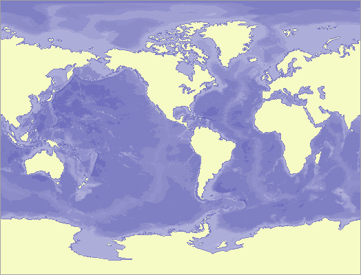
Figure 3: Seven Seas - A Geometry Object
The area computation program initialization consists of the
instantiation of the Voronoi grid as a memory-resident object and of
the steps necessary to establish the memory-mapping access to the
files containing the two objects. The area computation is packaged
as a Hipparchus Library function named h7_RsetAreaPerimeter();
its parameters are four pointers to given data: to the Voronoi grid
descriptor, some workspace, ellipsoid geometry parameters, and header
data of the object for which the area is required; plus two pointers
to returned values: the area and the perimeter.
The results presented here have been obtained using the code compiled
with the GNU C compiler V.2.95.2, carried out on a 400 MHz Pentium II under
Linux kernel 2.2.14. (Performance under NT was only marginally slower).
Ellipsoid: WGS 84, a=6378137.0e0, b=6356752.3141e0
The 2432 element cell-array area initialization took 0.19 seconds
and produced the following values (square meters):
Ellipsoid area:          510065621716336.1
Total area of all cells: 510065575723515.5
Difference:                     45992820.6
Relative difference (one in):   11090113.0
Area computation for both objects took 3.94 seconds (each),
and produced the following values (square meters, meters):
Landmass area: 150998900960532.0, perimeter: 1249923047.850
Oceans area:   359070890924373.1, perimeter: 1249923047.850

Ellipsoid area:          510065621716336.1
Landmass + Oceans        510069791884905.1
Difference:                   4170168569.0
Relative difference (one in):     122313.0
Conclusions
The following conclusions seem to be justified:
-
Computation of the ellipsoid cell areas using local mean curvature at
the cell center produced the results which are within one in 11 million
of the total ellipsoid surface area. For the grid and objects
as examined in the example, this is two orders of magnitude better
than the results of the object area computation, and thus adequate.
-
Computation of two very large planetary complement objects produces
results which are within one in 122 thousand of the total ellipsoid
surface area. The obtained level of accuracy is a result of a combination
of factors; the major one probably the inevitable rounding error in a
very large number of (over 1.3 million) of relatively narrow triangles.
The obtained accuracy compares favorably with that in many operational
systems which compute the areas in the plane - at the outset a significant
departure from the true object geometry.
-
The very short time needed to carry out the area computations of large objects
makes it practical to compute it only as and when this information is
required. This facilitates the system design in which the area of a
global object of any size and/or shape is not treated as an independent
attribute, but rather as only one in a repertoire of measures that can
be derived from its canonical geometry definition.
References
-
______, Digital Chart of the World (CD publication),
United States Defense Mapping Agency, Fairfax, VA 22031-2137. July 1992.
-
Bomford, G. Geodesy, London, Oxford University Press, 1975 ed.
-
Bowyer, A and Woodwark, J. A programmer's geometry, Sevenoaks, Butterworths, 1983.
-
Jordan, Eggert and Kneissl, Handbuch der Vermessungskunde (Band IV: Mathematische Geodaesie),
10th ed. Metzlersche Verlag., Stuttgart, 1959
-
Kimerling, A. J.Area Computation from Geodetic Coordinates on the Spheroid,
Surveying and Mapping, Vol. 44, No. 4, 1984, 343-51.
...